Image Processing and Quantification

Quantification of Planar Imaging

1. Background subtraction
1. Reduces tissue cross-talk and noise from the images
2. Bilinear interpolative background subtraction
3. Improve image quality by reducing cross-talk
4. Concern - Too much subtraction will remove myocardial tissue creating false defects
5. If the RV visualizes do not subtract out the RV


2. Smoothing - Is the next step
1. Standard 9-point weighted averaging
2. From the box below the counts of the center pixel is averaged with all the surrounding pixels, creating a 9-point smooth
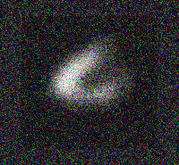
3. Creating a circumferential profile (refer to the three images)
1. First Image shows a 45 degree LAO



2. Second image shows a circle or ellipse is drawn around the LV with an arrow pointing at 0 degrees

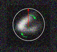
3. At the 0-degree within the circle the computer determines the maximum pixel count on 60 separate radii position as the profile rotates in a clockwise fashion around the myocardium
4. Then an activity curve is generated (see the next image) which displays maximum pixel counts around the LV for each of the 60radii
5. Note - The arrow "A" indicates an ischemic defect that fills in on the resting images



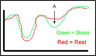
6. This procedure is done for stress and resting/redistribution images
7. Normalizing the images is also important and that is to assure that both sets of imagines have equivocal count presentation
1. Stress image may have an overall higher count rate
2. Rest/redistribution may have a lower count rate
3. Stress images are normalized to the rest/redistribution
8. Alignment of the initial profile is important in order to reproduce the data on both stress and rest/redistribution are the same
9. Stress and rest/redistribution images must also be taken at the exact same angle, otherwise generating the curves will misrepresented each other
4. Generation of Washout Rates Profiles (activity curves) - These terms apply to ²⁰¹Tl
1. The easy way to see if there is defect is to compare the stress curve to the rest/redistribution curve
1. If the stress segment on the curve shows less activity than in the rest/redistribution, ischemia is diagnosed (reversible defect)
2. If the stress segment and the rest/redistribution segment shows a significant drop in counts along the myocardial wall then infarct is noted (non-reversible defect)
3. If the stress segment is below the rest/redistribution segment on the curve then there is reverse-redistribution (non-transmural infarct)
2. Abnormal reduced washout rates can be noted when a section of the compared curves is greater than 2.5 standard deviations
3. Similar assessment can be applied with pertechnetate tracers


3. Processing and quantification of SPECT images (Using Philip's software)
1. Filtering and reconstruction
1. Each image is corrected for non-uniformity with a 30-million count correction flood (64 matrix)
2. If the matrix size is 128 then the correction flood should be 120-million
3. COR is applied to assure proper alignment of all images
4. Pre-filter the raw data is usually done with a 9-point weighted filter. Why pre-filter?
5. Images are then reconstructed with filtered backprojection protocol
6. During reconstruction images Butterworth filter, cut-off frequency of 0.2 cycles per pixel and an order of 5 may be applied. Or a Ramp an Hanning filter could be used. (we will cover this in greater detail in CLRS 322)
1. Changing the order will sharpen or smooth images as noted in the link
2. A low order gives a will make the image sharper and decrease background
3. A high order will increase background and give a smoother image
4. Do you understand points 2 and 3?
5. Issue finding the right order is very important and is somewhat system depended and must be determined by the individual person given the parameters of the imaging/computer system
7. Just a little bit more information about SPECT and filters link here (this data will be discussed in class)



2. From the raw data above tomographic images are processed via ADAC (Philip's) protocol



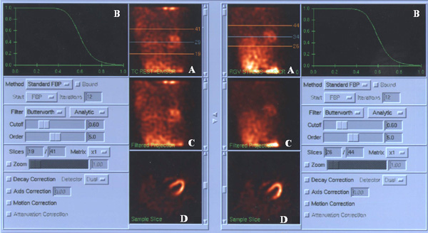
1. A - Images are displayed in cine format. Upper and lower regions are drawn above and below the LV. Every pixel within the these lines are processed and it is critical that ALL cardiac tissue is within these lines
2. B - Sets the Butterworth filter with cut off and order. Adjusting the cut-off and order will adjust the MTF curve
3. C - Is the same as A except that the regions are not drawn around the LV
4. D - Results of the reconstruction, showing the initial image which is the transverse image
5. Consider the tomographic slices see future lecture, "Anatomy of the Myocardium - SPECT and Planar"



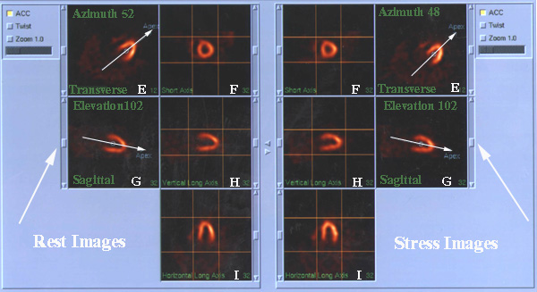
3. The program being used automatically sets all processing parameters and generates the Vertical Long, Horizontal Long, and Short Axis. If necessary, adjustments can be made
1. Adjusting the azimuth in the (E) the transverse image will adjust the angle of the Vertical and Horizontal Long. Angle should be the same for stress and rest where the arrow bisects the apex of the LV. Each processing step re-orientates the heart into the right plane for the next set of reconstruction
2. Adjusting the sagittal images' (G) affect how the other slices are generated. The same issue is in play, the degrees of elevation should be very similar
3. Adjustment may also be done to the short axis image (F) by adjusting the lines in the box. If there is background outside the LV, then the box can be adjusted to eliminate it from the processed data
4. The same concerns regarding the boxes around the Horizontal (I) and Vertical Long (H) apply (goal - cut off surrounding background if present)
5. Also note the sliding bar outside the imaging area (white arrows point to them). This allows you to page through all the slices in the short axis, vertical long, and horizontal long images
6. From the above discussion - what aspects of the processing should have been done differently?
4. Alternate approach to processing - Seimens software
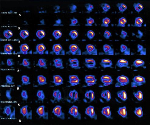
5. Displaying your results
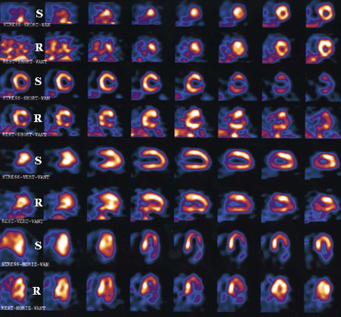
1. Case one is an example of multi-vessel disease of the LAD and RCA. Moderate to large amount of anteroseptal apical and small to moderate amount of inferolateral wall ischemia



2. Case two is a patient with partial defect shows a moderate sized inferoposterolateral myocardial infarction with a moderate amount of peri-infarctional ischemia. Mild inferoposterolateral hypokinesis. LV EF 64%



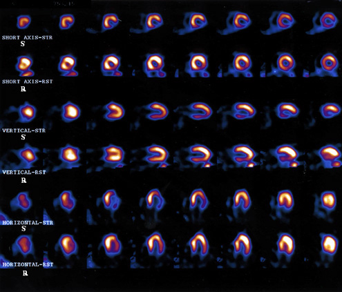
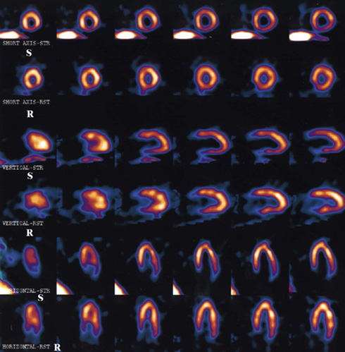
3. Case three shows infarct but no ischemia. Moderate sized inferolateral myocardial infarct. EF 60%. This was a dobutamine study



4. Case for is an example of a false positive study that initially looks like ischemia. However, the reduced activity to the myocardial wall on stress is do the computer picking the liver counts as the hottest pixels. The result is that the wall next to liver has reduced uptake. Note that the defect does fill in on delays. Corresponding to this is the lack of liver uptake next to the LV.