SPECT -
Attenuation Scatter and its Resolution
Lecture also includes two additional subcategories
1 - More on Scatter and Attenuation
2 - How does CT generate AC images - specific example relates this to PET
3 - Two objects with different amounts of activity - in the same plan
- Problems with photon attenuation
- Attenuation of photons by the body habitus makes it difficult to obtain accurate quantitative information. If fact, attenuation and scatter actually distorts the acquired data making quantification difficult
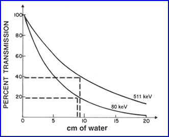
- As an example, in PET brain <40% of the photon actually make it out of the cranium. The reason for this is the that these photons have to travel though fluid media and from the center of the brain it may be up to 10 cm or more. This media attenuates, scattered, and absorbs the photons
- In a second example, 133Xe as seen above, with a less energetic gamma (81 keV) has approximately 20% of the gammas leaving the cranium when traveling 10 cm of water
- This information tell us - as photon energy increases attenuation and scatter decreases. Consider this point when comparing SPECT and PET and the types of radionuclides we use. Your thoughts on this?
- Broad vs. narrow beam geometry
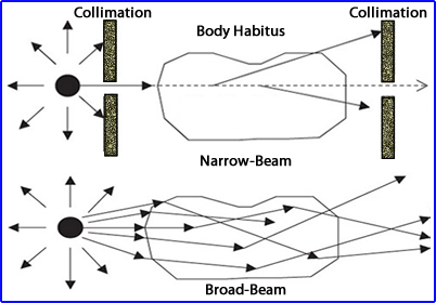
- When x or gamma rays travel through an attenuating environment there are processes to consider (broad and narrow beams)
- In the narrow beam approach the beam of radiation culminated results in a smaller amount being detected at the other end. The loss is do to scatter and attenuation
- Application of the broader beam shows the same effect but this time a lot more radiation gets through
- Key - The amount of radiation detect depends on: (1) the energy gamma being emitted and (2) the attenuating material's density
- As noted in other lectures - Attenuation (loss) occurs when gamma rays interact photoelectrically where and scatter occurs when gamma rays interact via Compton
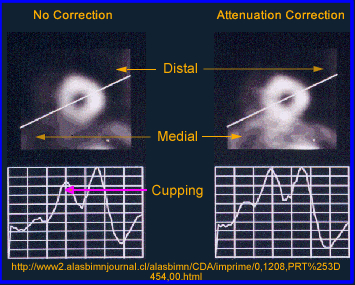
- How does distance of object, scatter, and attenuation effect SPECT? Let's evaluate the above image
- This demonstrates how depth affects resolution in terms of a line/point spread function
- The inner peak defines the geometry
- The middle "dotted" peak defines scatter
- The outer peak "solid line" blends the first two peaks
- This clearly shows us how depth alters spatial resolution based on the location of the radioactive source
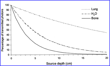
- From the source of the 99mTc gamma, the distance it travels, and the type of media encountered will alter the amount of attenuation and scatter. As noted in the above graph1
- The amount of scatter that occurs in SPECT can be anywhere between 20 to 50%. The end result? Is a loss in spatial resolution and image contrast - Why is this a true statement? Are scatter gammas counted within a PHA window?
- The author also defines a concept usually found in CT, beam hardness.
- This occurs when a beam of radiation encounters tissue(s) and becomes attenuated
- The lower lower energies are lost and more of the higher energy gamma (or x) rays make it out of the body habitus
- When discussing a polygenic emitter such as CT this concept can be more appreciated. However, if you are applying this to 99mTc, this is a monogenic gamma ray therefore beam hardening becomes more difficult a concept to apply. Can the same be said for 67Ga and 201Tl?
- Always apply the concept of linear attenuation coefficient with the density of the attenuating object and the energy gamma being associated with it - Why is this an important concept?
- Based on this data SPECT YOU must consider the following aspects of attenuation and scatter
- Consider the depth of the gamma-ray, its origin to the point where it reaches the detector
- Type of tissue(s) the gamma ray encounters before before it reaches the detector - attenuation
- Broad-beam attenuation characteristics as the gamma ray interacts with surrounding tissue
- Beam hardness as it relates to the attenuation properties of the tissue it encounters and the type of gamma ray being emitted
Application of μeff
- Measurements of photons being attenuated as a function of distance
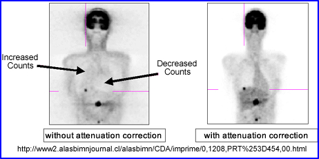
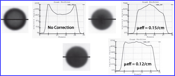
- The above image on the left defines activity without attenuation correction in which a count profile is drawn through the phantom of radioactive water. When AC is not applied there is greater loss counts at the center of a homogeneous volume of liquid. Additionally, the activity is more "hotly" distributed along the edge of the image causing an "edge packing artifact." Can you explain the type gamma interactions that caused type of appearance?
- Application of μeff = 0.15 is the value that represents the appropriate attenuation correction for narrow beam geometry.
- Notice that the image displays too much activity in the center which is reflected by the graph
- Consider - gamma-rays emitted do one come from a point source but from a media of liquid material
- = 0.12 reflects a broad beam geometry which most closely identifies a uniform uptake of activity, through the phantom and count profile
- This is the why AC should be utilized in the reconstruction process in a SPECT scan
- From a filtering standpoint the application of an attenuation correction can be mathematical, as long as the volume being imaged is homogeneous, such as the brain or may be certain areas of the abdomen
- However, if multiple densities are present then attenuation varies. This requires the application of a transmission source to determine the different underlining attenuation coefficients
- Type of a transmission source can either be a radioactive rod source attached to a fan-beam collimator or with an x-ray tube must typically CT
- Attenuation correction applied mathematically can either be done to the raw data (Sorensen filter) or during the reconstruction process (Chang filter)
- These types of filters are called first-order attenuation correction
- Can you apply one of these first order filters to correct for attenuation in an MPI procedure?
- Chang filter
- While this filter attempts to account for attenuation it does not take into consideration: scatter nor resolution at depth
- When the imaging media is at least somewhat uniform, the Chang filter is recommended. An attenuation map is based on the boundaries drawn around the patient skull were µ is constant. This generated a reconstructed transverse slices that are based with a µ of 0.15 cm or 0.12 cm-1)
- (A) Displays the reconstructed transverse slice of a 99mTc-HMPAO SPECT brain acquired in a 128 x 128 matrix. An elliptical ROI is drawn around the skull to define brain contour and the area to be corrected
- (B) A correction map is applied to the area inside the boundary and is given a value of 0.15 cm-1
- (C) Shows the brain SPECT without attenuation correction
- (D) Demonstrates the brain SPECT with correct
- The principle application to the process is that computer applies the attenuation correction factor (ACF) to each voxel in the 3D matrix and corrects for attenuation based on the depth of the associated voxel
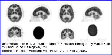
- Another example of the Chang filter being used is seen in the PET brain above
- Application of attenuation corrections with areas that have multiple densities
- When there is a variation of densities a line source or x-ray tube should be applied. With a transmission source one is able to define the different μ in the area of the acquired scan. How is this accomplished?
- Transmission based attenuation correction (TBAC) is the terminology used for this application
- Along with this data a reference scan of the transmission data must be obtained on every camera head. A reference scan is nothing more than checking the detector head(s) uniformity with the associated transmission source and generating the appropriate corrections. The reference scan is much like a uniformity correction matrix obtained by your 57Co flood. However, in this case we are correcting the transmission data
- Why is a reference scan important?
- Verifies that the transmission system is working correctly
- Line sources have brackets that support them and attenuate the beam being emitted. The reference scan corrects for this
- Finally, a reference scan should be done every day, especially if decay of the line source is a concern. Failure to acquire routine reference scan will cause an old reference to generate a falsely high correction
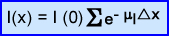
- The formula for AC is presented above
- μl represents each individual type of attenuation or linear attenuation coefficient
- e-μx is the attenuation factor within each segment rx
- I(0) is without attenuation
- I(x) presents the attenuated product
- Composition of an attenuation correction map
- What is an attenuation correction map? It generates attenuation coefficient values μ as variations in densities
occur in the corresponding voxels
- Each voxel then receives its appropriate correction by addition/subtraction/keeping the same amount of counts
- Consider the variation of bone, fat, muscle, and air .. how does the μ differ?
- These transmission images tend to be noisy which depends on the source generating the emission and the density of the attenuating body habitus - the weaker the source the greater the noise
- Shielding the aperture of the line source at its point of emission is also important. This may be necessary with a new source because it is to hot. This excessive activity will cause deadtime problems. As it decays the shield can be removed
- Noisy attenuation maps can be corrected by applying the camera's information density parameter, however, it is important to note the a very noisy image will cause error in AC
- Image segmentation can also be applied with the appropriate computer program, where the computer determines the type of tissue being attenuated and then applies a specific attenuation factor. Example - if it defines the tissue as bone then bone becomes the defining medium being attenuated. Bone, soft tissue, and lung are usually the only types of segments the system identifies
- Transmission Scans and camera designs with rod/line source
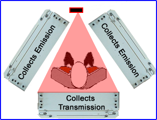
- Triple head configurations
- In this situation the line source sends data in one direction to collect the transmission data
- Two other heads acquire the gamma emissions
- Two-head configuration
- This configuration requires two line sources moving at the same time across the detectors' FOV
- Usually the transmission starts and finishes before the acquisition of the emission data
- In both configurations these line sources loss activity over time, requiring adjustments by increasing the acquisition time of the transmission source. Eventually it has to be replaced with a newer source
- Types of radioactive sources
- 153Gd is the most common source used with these imaging systems
- When initially installed the amount of activity ranges between 200 to 250 mCi
- Radiation dose given to the patient is around 0.4 to 25 mrem
- There is some concern to the radiation work since the surrounding area may have a background activity of 0.2 mR/hr
- Think about CT attenuation and how the room is setup at different clinicals in our area
- For Gd the major gamma emissions and K-shell characteristics x-rays occur between 40 to 103 keV
- In practical application, all radiopharmaceuticals used should be of higher keV so that transmission and emission peaks can be separated
- CT generated AC for SPECT
- In the procedure, when imaging, usually it starts with CT and then is followed by the SPECT scan. Rational is to reduce mis-registration
- Book states that the energy of CT x-ray must be similar to NMT procedure. This is not possible! The highest kVp I found was 150, with most CT scanner maxing out at around 140. So how does CT apply AC in a PET scan? Link to discuss this issue is found later in this lecture
- CT matrix is either 512 or 1024 so it must be down-sampled to 128 or 64. Regarding this how does it effect PVE?
- Segmentation can also be used in this approach and it is similar to what we just learned with transmission imaging (rod source)
- With CT, noise should not be an issue because the energy flux has stronger transmission imaging (plus no decay)
- AC maps and iterative reconstruction
- AC map is placed into the forward-projection step, in the EM process. μ is calculated for each voxel
- AC map is also used to estimate scatter
- Scatter compensation (SC)
- A thought - AC is used to increase the number of counts where there is a high attenuation coefficient and if there is a lot of scatter, then not only are you increasing your true counts, but also increasing bad data
- How do we deal with scatter?
- (Method 1) - Determine the scatter fraction
- If several windows are set below peak 20% window then faction(s) of scatter can be determined which in turn can be applied to correct the scatter in any given pixel
- This scatter is subtracted from each pixels in each the 2D matrix, reducing the amount of counts per pixel. Does this increase noise?
- Another problem with this relates to the 3D matrix. The further away from the detector is from the object of acquisition the greater the amount of scatter generated. Hence the problem with this method is that it does not take depth into account
- (Method 2) - Scatter and the iterative approach
- A phantom is used to measure the effects of gamma emissions at different depths as well as with different tissue types
- This data is then applied to the attenuation map in IR reconstruction at the forward-projection step
- There is an apparent 10 - 20% improvement in contrast when compared to method 1
- Resolution recovery (RR)
- Recovery filters
- The gamma camera acts similar to a low-pass filter in that it blurs an image (doesn't show structure like CT) which resembles a low pass MTF curve
- To remove the blur, the camera's MTF is deconvoluted, similar to applying Metz or Wiener filter
- The middle frequencies of the deconvoluted curve are then multiplied by a factor greater than one
- Noise is removed and trues counts are enhanced
- Low pass filter must be combined with recovery filter to suppress noise (can you give an example of a low pass filter?)
- Filter characteristics
- Metz utilizes the MTF as it relates to collimation and camera acquisition
- Wiener applies a signal-to-noise ratio (SNR) to different types of acquisitions parameters
- Problem: the process in which these filters are actually applied have some uncertainty and may not given true data nor it might not be appropriate for quantitative analysis
- Three methods that can be applied with IR where RR is applied
- Method -1
- Loss resolution is treated with the camera's FWHM @ 10 cm
- Data above 10 cm is over corrected
- Data under 10 cm is under corrected
- Method -2
- Incremental levels of depth and its associated FWHM are applied
- Evaluated at each slice and applied to the 3D matrix
- Method - 3
- Deconvolutes the 2D and/or 3D data to improve the resolution
- This is either applied during backprojection with FBP or forward-projection in IR
- Technical results with application of AC, SC, and RR
- Spatial resolution can be enhanced by x2 or more with FWHM seen around 4-5 mm vs. 10mm. Contrast has also been improved
- It seems that RR is the bases in which AC and SC rely on
- Key - We need to be able to accurately define the relationship between the amount of activity at different depths within a 2D projection. Knowing this we can determine the amount of attenuation that contributes to scatter
- Clinical points of interest
- AC correction does not seem to be the key to correcting and improving image resolution and contrast. SC and RR need to be integrated into this role if you really want to make work
- If the image quality can be improved via SC and RR that results in two times the improvement. Via
- Improve the ability to find disease via better resolution or
- Reduce our imaging time by 1/2
- Anatomical correction with CT along with physiological data improves patient outcomes. SPECT's spatial resolution is around 10-15 mm. CT's resolution can be reduced to 4-5 mm or less. End result with the combination is that diagnostic imaging improves
More on attenuation and scatter
- The counts in SPECT reconstructed images are, in theory, directly proportional to the absolute concentration of radiopharmaceutical in the organ or organ system of interest (e.g., mCi/cc or MBq/cc)
- The 2 main factors that prevent SPECT from achieving a quantitative goal relates to gamma rays inside the body interact with attenuation and Compton scatter prior to exiting. These 2 phenomena cause spatial distortion of the measured amount of injected activity, hence effecting the ability to quantify the image
- Attenuation reduces the total amount of counts being collected
- Compton scatter reduces the amount of counts being collected
- Scatter can add to counts that are unwanted
- Attenuation
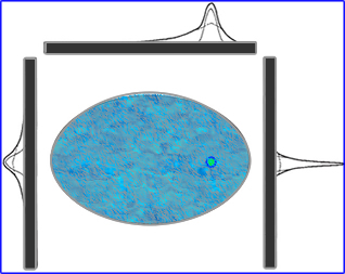
- For a given concentration of radioactivity the relative number of gamma rays that escape the attenuating medium and those that are detected by the gamma camera can be determined by this equation:
where:
- I = the attenuated intensity of gamma arrays
- Io is the gamma-array emission intensity without attenuation
- µ = the linear attenuation coefficient of the medium (for example, approximately 0.15 cm-1 for 99mTc in soft tissue)
- lq = the depth of the medium between the source of activity and the gamma camera at projection angle q
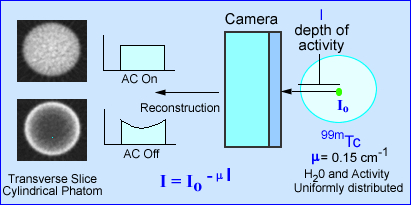
- The effects of attenuation on SPECT imaging is further noted in the above image. The intensity of photons emerging from a source (cylindrical phantom) of activity has a given amount of attenuation, water, that reduces the amount of gamma emission. The value e -µl, in the formula identifies µ as the linear attenuation coefficient in cm-1 and l as the depth of the activity in the attenuating medium. This is based on a specific projection
- When attenuation correction (AC) is off a cupping artifact in seen in transverse reconstructed image. The explanation of the cold center occurs because of the attenuated gammas. If fact the closer to the center of the cylinder the greater attenuation. However, if AC is turned on the there is an equal distribution of activity across the entire transverse slice
- In SPECT studies dominated by soft tissue attenuation may required the application of, µ, which can be done by using a filter, such as Chang. A value of 0.15 cm-1 is applied since soft tissue attenuation has the same density as water
- When soft tissue is combine with air and/or bone (i.e. lungs) the attenuation phenomenon becomes too complicated to handle the attenuation from a mathematical standpoint. It is in this type of situation that a transmission scan is needed to account for the attenuation variations
- Attenuation correction methods may be categorized as:
- Constant µ, or the Chang method
- Variable µ, or transmission source method
- When the imaging media is at least somewhat uniform, the Chang filter is recommended. An attenuation map is based on the boundaries drawn around the patient skull were the constant µ is applied. This generated reconstructed transverse slices. ( µ = 0.15 cm-1)
- Now let is consider variable attenuation coefficient which is dependent on the spatial location of the pixel in the patient
- The quantitative value of µ is determined by the use of transmission scanning, either by use of a line sources , or x-ray transmission
- From the transmission scan, a µ map is generated, which is the inverse of the attenuation correction factor
- Transmission sources are long-lived radioisotopes that should have energies similar to the radioisotope being acquired. 153Gd (100 keV) maybe preferred for 201T while 57Co (122 and 136 keV) might be preferred with 99mTc. The correction factors are then converted to the attenuation coefficient map from the transmission data.
- In the above image the image on PET brain scan on the left uses a attenuation map generated from a single µ value. The image on the right uses a 137Cs source for its attenuation correction. Do you see a difference between both procedures? If so, where?
- The accuracy of the transmission source attenuation correction methods depends on the strength of the transmission source, lack of patient motion, and the attenuation correction algorithm itself
- Variable µ attenuation correction may be best performed using iterative reconstruction methodology, but can also applied to filtered backprojection.
- The clinical accuracy of transmission scanning methods in perfusion SPECT imaging is currently the subject of controversy. Attenuation correction has been shown to be of some use, but complete correction in all patient studies still eludes this technology
- From my own personal experience in nuclear cardiology (my opinion) is that variable attenuation correction does not greatly improve the diagnostic ability of the procedure. The problem may have been that motion correction could be applied to the emission data, could not be applied to the transmission (GE software). If the programs now allow for motion correction of the transmission and emission data my guess is that it might significantly improve this correction technique
- Yet another example of the application of transmission data is seen in the above PET scan. What seems improved? Check the background activity. Check image resolution
- Compton Scatter
- The finite energy and spatial resolution of the SPECT imaging system allow for the acceptance of a certain amount of Compton scatter gamma rays (8 - 12%).
.
.
- The accepted scatter is dominated by narrow angle scattered gamma rays, which interact with orbital electrons and have energies slightly less than that of pure photopeak gamma rays, but are within lower end of the window. Note the red scatter line
- Compton scatter degrades resolution and acts as a modifier to the effective attenuation coefficients in a depth dependent fashion. Moreover, misplaced Compton scattered events adversely effect image contrast. Contrast is effected because false data is being accepted in the counting window
- Some SPECT systems include scatter correction methods based on the physics and probability of the Compton scatter process by using multiple or weighted energy window. An method to consider for Compton correction:
- Collect two separate photo peaks
- The first peak is set to the energy gamma (A) and the second is set to Compton peak (B)
- A - B = an energy peak with reduced Compton scatter
- In the future, improved energy resolution and window acquisition methods, and iterative reconstruction methods will include Compton scatter modeling
- Attenuation correction
- Filters have been designed to take attenuation into account
- The only problem with this approach is that the user can only apply this to areas of the body where the body habitus density remains relatively constant (brain and liver)
.
- Why should attenuation be taken into account? Remember the cupping artifact? Graphically the above example shows the affects of cupping in the LV of the myocardium. A profile is drawn through heart and a decreased in counts can be seen in the septal wall. Can you explain this artifact?
- The two types of attenuation filters are used in nuclear medicine: Chang (applied post reconstruction) and Sorensen (applied prior to reconstruction)
- The Chang method starts by drawing an ROI around the widest portion of the transverse slice. Once defined an attenuation value is then given to the data and a correction in counts is applied to the pixels inside the ROI. In theory this increases the counts coming from the center of the image negating the cupping artifact. Remember - the closer to the center of the brain (or any organ) the greater the gamma attenuation and the greater the need for correction
- Water has a µ value of 0.15 cm-1 which is applied to all liver brain and liver attenuation filters
.
- While attenuation correct filters are sometimes used to improve image quality this process cannot be done if there are different areas of density within the FOV. At this point only a transmission source can be used to compensate for the differences in density within the imaging media. Example of this would include the myocardium and bone
- Transmission imaging can be accomplished with the use of a line source and a fan beam collimator or with an x-ray tube (CT)
How does CT apply Attenuation Correction to a Nuclear Study?
- Application of CT Attenuation with PET (can also be applied to SPECT - especially with higher keV gammas) images
- We will discuss one of several methods used to correct attenuation densities in a PET scan. PE Kinahan and his associates discuss the development and application of CT attenuation and its role with in PET
- What is scaling and why does it need to be applied in CT attenuation?
- 511 keV gammas for PET interact differently than its CT counterpart (70 - 140 kVp)
- Reason - First there is greater attenuation with lower energy x-ray. In this energy range, when compared to PET gammas, there is greater photoelectric and Compton interaction. On the other hand because of PET gamma rays have a significantly higher energy there is less Photoelectric and Compton interaction.
- When comparing PET to CT the probability of x-rays interacting with air, water, and soft tissue is approximately 1.9. Furthermore, Photoelectric effect increases by 13% when CT x-rays encounter bone, while PET gamma rays increase by just 3%.
- Why do x-rays and gamma ray interactions increase in the Photoelectric range when encountering bone? (1) the presence of calcium and phosphorous in the bone and (2) these elements have higher Z values when compared to the surrounding media
- Therefore, it is important to scale CT x-ray for proper correlation of attenuation in the 511 keV range
- Monochromatic gamma vs. polychromatic x-ray
- PET gamma rays always have the exact same energy, 511 keV
- CT x-rays vary in their energy beam, even when it is set at a specific energy level. Usually there is at least a 1% variation within any given setting. This fluctuation causes a slight variation within any given attenuation coefficient
- Segmentation
- This is a process in which attenuated CT values are converted to known μ values of specific tissues found in the body
- Given a certain threshold with the CT x-ray the specific tissue type is identified
- In general, there is a choice between μ bone, soft tissue, and lung
- One minor problem with this approach occur when certain types of tissue have variation in density
- As an example consider the lungs. Within the thorax you will encounter soft tissue (heart), lung (has air), and ribs (bone)
- Once the different tissue types are identified Scaling and Segmentation are applied
- Segmentation defines the specific organ or tissue type and applies the correct attenuation
- Scaling (ratios) for bone, soft tissue, and air will further adjusts the attenuation map to the 511keV gamma
- General application of attenuated maps in PET
- Increased density translates to higher CT attenuation coefficients which in turn will increase the amount of counts in the same region of the corrected PET images
- Decreased density translates to lower CT attenuation coefficients that will reduce the amount of counts in the corrected PET image
- It is very important that Co-registration of CT and PET occur for appropriate pixel to pixel alignment
- Matrix size must be adjusted. Remember CT has 512 x 512 and PET has 128 x 128
- Artifacts occur when there is a density mismatch
- Remember to always look at your raw data: CT and PET
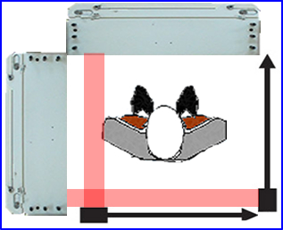
Two objects of different activity levels along the same ray
- Measuring/imaging hot spots with varying amounts of activity in different location (depths) along the same ray(s) is another problem that needs to evaluated (see above example)
- C is the detector head collecting counts at a specific angle (ray)
- The hottest source of radiation is at the most extreme point, S1 and has a distance, Da, from C
- Another source of radiation is a lot closer to the camera, but is has less activity, S2 and its distance, Db, from C
- Considering the distances and appreciate that the attenuation will be greater with S1 when compared to S2
- Is there an issue with two sources at varying distances?
- What if S1 has significantly more activity when compared to S2? Would this affect the SPECT acquisition?
- Acquisition data become mixed with the varying degrees of activity and differing amounts of attenuation altering the true amount of counts in SPECT. One should conclude that this problem does effect quantitative analysis
Return to the Table of Content
4/23
Determination of the Attenuation Map in Emission Tomography, H Zaidi and B Hasegawa, JNM vol.44 No.2 pp.291-315 (2003)