I am not interested in an item-by-item analysis of this scale. Instead I constructed an additive scale of "Pride in America" by summing up the responses to the ten items. A "scalability analysis" of the items shows that each one is correlated at least 0.4 with the sum of the other nine; the Cronbach alpha coefficient is 0.83. This coefficient is a correlation-type measure of the internal consistency of the scale, a generalized split-half reliability coefficient. To make the scale more easily interpretable I adjusted the sum so that the maximum value was 100 if the respondent said "Very Proud" to all 10 items, and its minimum was 0, if all ten responses were "Not at All Proud". For those of you who like algebra, the Compute formula is:
PRIDE = 100*(40 - SUM)/30
Comment: In SPSS the compute function "SUM(X1,X2, . . . ,X10)" will compute the sum of all non-missing values on any of the variables. To include only cases where responses to all ten items were valid, I used the function "SUM.10(X1,X2,X3, . . . ,X10)".
The distribution of values of the scale PRIDE has mean 70 and standard deviation 15, with noticeable outliers at the low end. I will ignore the outliers for now, but it would undoubtedly be wise to examine them at some point.

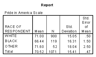
Let's see how the responses to this scale are related to gender, race and political party identification. In its original form the latter variable (partyid), has seven categories, ranging from strong democrat to strong republican. As you can see from the following tables of subgroup means, the strong democrats and strong republicans both show the highest degree of pride in America, while the independents show the lowest.


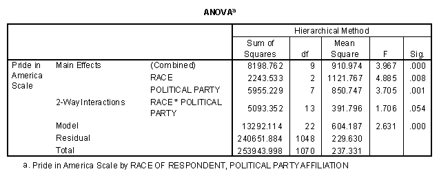
The three one-way ANOVA tables all show significance at the .02 level or less (the P-value for sex is .012). The two-way ANOVA on race and partyid gives the following results.

To begin with, note that the ANOVA table has several rows, some of which are nested within others. The rows for "model" "residual" and "total" are precisely what we would see if we had done a oneway ANOVA on the full 24 cell, grouping of the sample by race and partyid. The degrees of freedom for the model (between groups) are 22 rather than 23 because one of the 22 cells has zero observations, as the next table below shows. The model SS is the sum of the entries for race, partyid (the two main effects) and interaction. The ANOVA is described as hierarchical because each effect has been evaluated assuming that the previous effects have already been included in the model. Thus the table tells us that the 3 category race variable is, by itself, a significant predictor of pride (P = .008); party identification adds significantly to the predictability of pride (P = .001), and their interaction adds a little more predictability (P = .054). While the output of this SPSS procedure did not calculate the R-square values at each step, this can be done easily by taking appropriate ratios of the SS at each step to the total sum of squares.
To see what happens when the main effect for party identification is entered first into the model, I just change the order of the predictors in the SPSS command window. The resulting ANOVA table contains many of the same numbers. The one new piece of information in this table tells me that race is still an important predictor of pride in America, even after political affiliation has been controlled for.
The mean values and frequency counts in each of the 24 subgroups defined by the cross-tabulation of race with party identification are shown in the table entitles "Cell Means." Note that the Other Race, Other Party cell of the table is empty. The fact that White Strong Republicans have one of the highest mean levels of Pride in America, while Black Strong Republicans have the lowest mean level would be an exciting and unexpected finding, if it were not for the fact that there are only two respondents in the Black, Strong Republican category!


To carry out the regression analysis that is equivalent to this analysis of variance I need to create many indicator variables: at least as many as the number of degrees of freedom in the model (22). To begin with I would define Black and Other Race indicators, figuring that my best story would come from comparisons of these groups to the dominant "white" group. Next, I would define indicators for each of the party identification categories except Independents. That way regression coefficients would allow for contrasts of particular groups to the (presumed) center of the political spectrum. Defining the 13 or 14 indicators needed for the interaction terms is trickier, if I want the resulting regression coefficients to be easily interpretable. I can, however, just take the 14 product variables defined by multiplying each of the 2 race indicators by each of the 7 party indicators I have already created.


The two tables above show what happens when the race indicators and then the party identification indicators are entered into the multiple regression procedure of SPSS. The entries in the ANOVA table are the same as those in the first ANOVA table I reported, though they are arranged differently. The R-squared table is useful. The regression routine, of course, gives us more detailed information about the individual categories of race and party identification. The individual regression coefficients provide us with measures of the effect of being in one group or another, compared with other groups. The significance tests on the coefficients are t-tests of contrasts, in the jargon of analysis of variance.
Among other things, I can see that the Other Race group has about the same level of pride as whites do, whether party is controlled or not (P-values .68 and .78, respectively). That indicator could be dropped from the model. Likewise, when race is controlled for, the republican-leaning independents and democrat-leaning independents cannot be distinguished from the centrist independents (P = .84 and .95 respectively). In effect, we may simply collapse these response categories into a single "independent" category, as Agresti and Finlay did in their example in Chapter 12.
Having a strong commitment to one party or the other does make a difference, however, controlling for race. These conclusions could, in a general way, be made by looking at the table of means, but the regression analysis allows us to use the significance test logic more easily.

In order to see what the no-interaction model looks like when non-significant indicators are removed, I next entered all nine predictors and had SPSS perform a "backwards" analysis, dropping the least significant term at each step. The table that follows shows two of these reduced models. While it does contain a term with P > .05, I prefer Model 5 because the symmetric use of the party labels makes it a little easier to discuss. All these models have virtually the same value of R-square.
Finally, I used the General Linear Model, Univariate (GLM) procedure within SPSS, which produces output similar to what Agresti and Finlay show in Chapter 12. This output combines aspects of the regression and ANOVA approaches, by arbitrarily selecting one category of each discrete predictor variable (factor) to omit from the regression equation. I don't have to create any indicator variables, but still get the regression coefficients that would correspond to the indicator variables. I specified the "Type I Sum of Squares" option, which is the same as the hierarchical method I used earlier (and which I recommend using whenever possible). Race was entered first, then party identification, and then the interactions, consistent with the previous multiple regression analysis. As you can see, adding the interaction terms to the main effect terms increased the R-square from .032 to .052, and the adjusted R-square from .024 to .032. Removing the many non-significant terms from the model would decrease the model's degrees of freedom. It would make little difference in the R-square, but would increase the adjusted R-square. (Adjusted R-square will increase whenever a variable with a t-coefficient less than 1 in magnitude is removed from a regression model.)


The regression coefficients in the model that includes all the possible interaction terms are quite different than the ones in the model that only contains main effect coefficients for race and party identification. One message that I hope it conveys is the impossibility of speaking of "the effect" of a predictor variable in a complex model that involves interaction terms, nonlinear terms, and/or variables whose causal connection to the predictor is unknown.
