Example 6: Space-curve plotting,
parametric curves
Objective: Plot and analyze the
space curve given parametrically by the following equations:
x = 2cos(3t), y = 2sin(3t),
z = 3sin(t)
The DPGraph Commands: Click here to download the .dpg file
on your computer for a list of commands used in the correct
syntax and for later modifications. Note the use of parentheses
(to clarify operations) and asterisks (for multiplication). Also
note the following:
Unlike standard graphics calculators or
the textbook, DPGraph uses the letter "u"
instead of "t" for the parameter.
The order in which the coordinates appear
inside the "rectangular(...)" command is
interpreted by the DPGraph as the standard order: x,
then y, then z.
Given that the term "sin(u)"
has the longest period of 2*pi in the three
components, the first two of the following commands:
GRAPH3D.MINIMUMU := 0
GRAPH3D.MAXIMUMU := 2*PI
GRAPH3D.STEPSU := 100
display the graph of the entire space
curve over the parameter range u in the
interval [0,2*pi]. This is a bounded curve
since the trigonometric functions that define its coordinates
are all bounded functions. A bounded curve can be fully
plotted inside a finite viewing box.
The third or bottom command ensures that the
graph is smooth by using a sufficiently high number
of "u steps" (try re-drawing the curve
using a smaller number than 100, say, 30; the resulting
non-smooth curve is wrong! On the other hand, once a
smooth curve is obtained with say, 100, larger step values
are inefficient and should be avoided). Figures 1,
(A) and (B) shows the same curve from two different view
points.
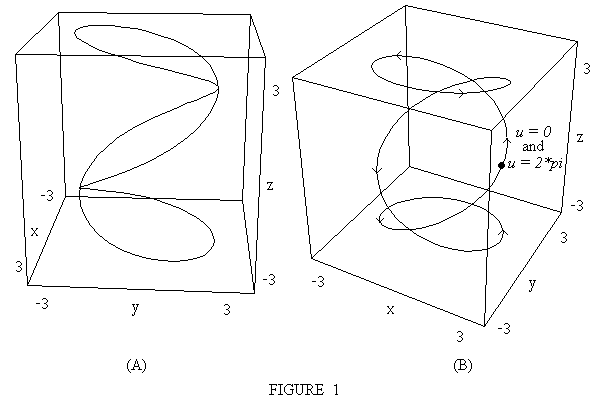
Note that although in Figure 1(B) the curve appears
to itersect itself 6 times, Figure 1(A) shows that it actually
does so only 2 times. Can you find these points graphically?
Analytically?
Analysis:
To Determine the orientation of
the curve as shown in Figure 1(B), adjust the
GRAPH3D.MAXIMUMU command to a number close to zero, and
redraw the graph; note which part of the curve is drawn
and use this observation to determine the correct
direction on the curve. Note also from the given
equations for the curve, that when u = t = 0, we
obtain the point (2,0,0) on the curve, and this
same point is obtained when u = t = 2*pi.
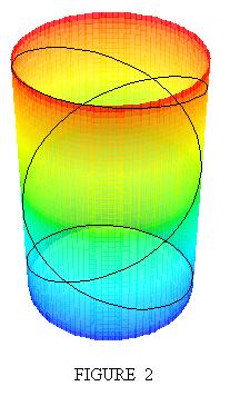
The curve lies on and wraps around a
right circular cylinder (or a "pipe") of
radius 2. This is easily seen by computing:
x^2 + y^2 = 4([cos(3t)]^2 +[sin(3t)]^2) = 4
which is the familiar equation of the
cylinder in rectangular coordinates. By drawing and rendering
the cylinder separately using DPGraph, and then superimposing
the curve on the cylinder in MS Paint, we obtain the
following figure which verifies our conclusions:
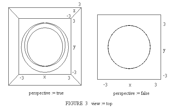
Another way of seeing the
wrap-around-the-pipe feature of the curve, is by looking at
it from above. This is done by adding the command:
GRAPH3D.VIEW := TOP
which gives the graph on the left in Figure 3
below. We see both the circularity and the two
self-intersection points in this graph. The graph on the
right is obtained by adding an extra command,
GRAPH3D.PERSPECTIVE := FALSE
that turns off the 3D perspective.
In this case, we do not see the bottom of the cylinder as
being farther from us, hence appearing smaller than
the top; both top and bottom are treated equally when there
is no 3D perspective and we clearly see the circular boundary
of the cylinder that contains the curve (no longer visible)
in it.
To find the length of the curve,
it is necessary to use the arc-length formula and
integrate from 0 to 2*pi. This may be
done using the MPP software, or alternately, on the TI-83
(and similar) graphics calculator as follows:
Enter the appropriate functions into
the arc-length formula, and simplify as much as
possible to conclude that the length of the curve is
obtained by integrating the square root of 4 +
[cos(t)]^2 from 0
to pi, and then multiplying the answer by 6.
Enter the square root of 4 +
[cos(x)]^2 as
function "Y1" into the TI-83, noting that
the calculator uses x as the standard
variable, not t.
Set the calculator "window"
large enough that the graph of Y1 is fully visible
(if not sure, graph Y1 first).
Press [2nd] [trace] to access the
[calc] menu, then press [7] for the integral (or
scroll down to it, then press [enter]). The
calculator draws the graph and prompts for a
"lower limit?" Enter 0 or move the
cursor to 0, then press [enter]. When the
calculator prompts for the "upper limit?"
enter 3.14 for pi (it seems that
TI-83 accepts only two decimal places; for more
accurate results, you need to move the cursor
manually, or use the MPP software). Pressing [enter]
again should give an answer of about 39.94
(after rounding to two decimal places) for the length
of our curve.